Benchmarking in Power Pivot with NAV

When working with sales data it is often required to calculate values against a certain benchmark. If available, using budgets is certainly the best option. In many situations this is however not an option since even the best managed budgets cannot be available on all possible reporting levels. This post will show alternatives to manually created budgets by using DAX-calculations that take the past into consideration to calculate a benchmark for the future.

The idea is to use values from the past to benchmark the present against those figures. Rolling averages are often used to see trends over time. Using rolling averages has been well described here and here. However, in businesses that have the tendency to show strong seasonal trends (construction business, fashion etc.) this type of average does not help a lot.

The simplest and most often used benchmark that takes seasonality into account is the value of the same period last year. However if not only the same period last year should act as source of the benchmark but the same period of multiple years in the past, another average is more meaningful. This blog post will explain how to define the average sales of the same month during the last couple of years. Since it obviously makes a difference how many years in the past should be considered we want to allow the user to select the number of years in a slicer.

The following video shows the general idea and what the solution could look like in a Cronus Extended database.

[video width="924" height="472" mp4="http://www.navida.eu/wp/wp-content/uploads/2014/08/AveragenYears1.mp4"][/video]

First, we need to retrieve the sales data from NAV. We start with a simple data model based on a NAV query that returns all posted sales invoices (headers and lines):

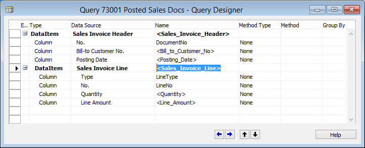
Based on this query and two simple OData-Feeds for customers and a date table we create the following data model:

What we want to do is to create three measures – sales for the sales of the current month, average sales of the last n months and a derived measure that shows the difference in % - the deviation from actual to benchmark.

First we create a simple linked table in Excel that will be used as the source of the slicer that allows to change the number of years to take into consideration:

Sales is the simplest measures defined as

Sales :=
SUM ( [Line_Amount] )

We had to add the following calculated column to our date table that provides us with a sequential list of month numbers that we can use to jump back one or multiple years since DAX is (as far as we know) lacking such a time-related function right now:

Before creating the measure that shows the average according to the slicer selection it may make sense to see how we would calculate the sales of the last year using our calculated column:

SalesBefore12M :=
CALCULATE ([Sales];
FILTER (
ALL ( DateTable );
DateTable[Months relative]
= MAX ( DateTable[Months relative] ) + 12
)
)

As usually CALCULATE is the main function here – it shifts the date context by 12 months.

Since we want to see the average not only for the same month last year (that would actually be no “real” average) we need to calculate the average of the number of years according to the slicer selection. The following measure that leverages SUMX does the trick:

salesBeforeXM :=
SUMX (
VALUES ( YearView[Year view (intern)] );
CALCULATE (
[Sales];
FILTER (
ALL (DateTable );
DateTable[Months relative]
= MAX ( DateTable[Months relative] )+ YearView[Year view (intern)] * 12
)
)
)

Here we use the second column of our linked table YearView[Year view(intern)] to retrieve all those years that match the slicer selection. If the user for example selects the value 2 on the slicer, that linked table would be filtered to

SUMX would perform the inner calculation twice – once with Year View (intern) 1 and once with value 2. This would result in a sum of the sales of one year (12 months) and two years (24 months) in the past. Since we are interested in the average and not the sum, we need to divide this by the number of years that we looked into the past.

AvgSalesBeforeXM :=
IF (
[Sales] > 0;
DIVIDE (
[salesBeforeXM];
COUNTX (
VALUES ( YearView[Year view (intern)] );
CALCULATE (
[Sales];
FILTER (
ALL ( DateTable );
DateTable[Months relative]
= MAX ( DateTable[Months relative] )
+ YearView[Year view (intern)] * 12
)
)
)
)
)

The deviation would be just the ratio of the difference between sales and average and the current sales:

% Deviation To Average :=
IF (
AND ( [AvgSalesBeforeXM] > 0; [Sales] > 0);
DIVIDE ( [Sales] - [AvgSalesBeforeXM]; [Sales] )
)

On a Cronus, the result could look like the following - first with a look-back period of one year...

...and with a look-back of three years...

In some cases, a moving weighted average (linear or exponential) could provide better results if the near past should be weighted stronger but even this simple approach may provide a good first baseline for performance-benchmarking.